
Cygwin and Cygwin X Terminal
Start Cygwin
To start Cygwin,
- Press the Windows key
 + s key (search command).
 - Type Cygwin.
- Select Cygwin64 Terminal.
A Cygwin64 Terminal will appear.
Start Cygwin X Terminal
Gnuplot requires X Window System to display. We just start X Server and launch an X Terminal.
First, create a new .XWinrc file in your home directory (note that there is a leading period in the file name):
On Cygwin64 Terminal, run the following commands to check if .XWinrc file exists:
cd
ls -la .XWinrc
If .XWinrc file exists, backup it:
mv .XWinrc .XWinrc.org
Then create a new .XWinrc file:
cat>.XWinrc
And type the followings on Cygwin64 Terminal (suppose that your Cygwin is installed in c:\cygwin64). Do not use Japanese characters, including the Space.
ICONDIRECTORY c:\cygwin64
ICONS {
  xterm Cygwin.ico
}
menu root {
  Xterm exec "mintty"
}
RootMenu root
SilentExit
In Cygwin64 Terminal, type Ctrl key + d key to terminate input.
You can check the contents of .XWinrc by executing the following commands on Cygwin64 Terminal:
pwd
ls -ltra
cat .XWinrc
Then start X by executing the following command:
xwin -multiwindow +iglx -clipboard -xkblayout jp -xkbmodel jp106 &
A Cygwin/X Server icon will appear in the taskbar.
To launch an X Terminal, right click the icon of the Cygwin/X Server and select Xterm.
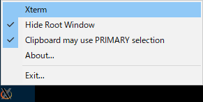
An X Terminal will appear. If there is no Xterm item in the menu, your .XWinrc may contain contents with wrong formats.
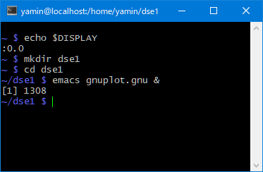
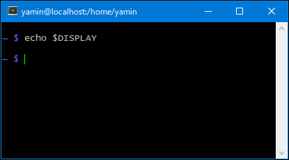
You can type the command echo $DISPLAY. The X Terminal will echo ":0.0".
Gnuplot Templates
Gnuplot Example
In X Terminal, run the following commands to prepare the gnuplot.gnu file:
mkdir dse1
cd dse1
emacs gnuplot.gnu &
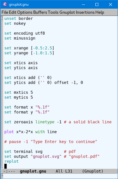
An emacs window will appear. Add the following codes to the emacs window. You can use Ctrl key + y key to paste copied characters in the emacs window.
unset border
set nokey

set encoding utf8
set minussign

set xrange [-0.5:2.5]
set yrange [-1.0:1.5]

set xtics axis
set ytics axis

set xtics add ('' 0)
set ytics add ('' 0) offset -1, 0

set mxtics 5
set mytics 5

set format x "%.1f"
set format y "%.1f"

set zeroaxis linetype -1 # a solid black line

plot x*x-2*x with line

# pause -1 "Type Enter key to continue"

set terminal svg         # pdf
set output "gnuplot.svg" # "gnuplot.pdf"
replot
In emacs window, type Ctrl key + x key, Ctrl key + s key to save the file.
On X Terminal, run the following commands:
ls -ltr
gnuplot gnuplot.gnu
ls -ltr
You will see that the gnuplot.svg file was generated. You can also set output to PDF format.
Gnuplot Result
Open a Windows folder for the current directory:
cygstart .
Then open gnuplot.svg with Mozilla Firefox, Google Chrome, or Microsoft Edge or IE.
You can insert gnuplot.svg to your Microsoft Word or PowerPoint (Office365) file.
Gnuplot Time Complexity
Below is another example. File name is BigO.gnu. You can use emacs to edit it
set xlabel "x"
set ylabel "f(x)"

set xrange [0:10]
set yrange [0.001:10000]

set xtics 0, 1, 10
set mxtics 2

set logscale y
set key at 9.5,1.0

plot log(x)/log(2)   title "log_2(x)",\
     sqrt(x)         title "x^{1/2}",\
     x               title "x",\
     x*log(x)/log(2) title "x log_2(x)",\
     x*x             title "x^2",\
     x*x*x           title "x^3",\
     2**x            title "2^x",\
     int(x)!         title "x!"

set terminal svg      # pdf
set output "BigO.svg" # "BigO.pdf"
replot
Run BigO.gnu
gnuplot BigO.gnu
Generated BigO.svg (transparent)

Gnuplot Data File
gnu_plot_data.gnu. It plots data from file latency.dat.
set xlabel "Traffic load"
set ylabel "Latency (cycles)"

set format x "%.1f"
set format y "%g"

set xrange [0.05:0.5]
set xtics 0.0,0.1,0.5

set yrange [240:710]
set ytics 250,50,700

set mxtics 2
set mytics 5

set key at 0.25,650

plot "latency.dat" using 1:2 title "Algo. 1 on workload 1" with linespoints, \
     "latency.dat" using 1:3 title "Algo. 2 on workload 1" with linespoints, \
     "latency.dat" using 1:4 title "Algo. 1 on workload 2" with linespoints, \
     "latency.dat" using 1:5 title "Algo. 2 on workload 2" with linespoints

set terminal svg               # pdf
set output "gnu_plot_data.svg" # "gnu_plot_data.pdf"
replot
latency.dat
#1	2	3	4	5	col# gnuplot
#0	1	2	3	4	col# pyplot
#p	A11	A21	A12	A22
.05	285	270	312	288
.10	287	272	328	296
.15	291	275	338	308
.20	312	292	353	321
.25	347	323	370	339
.30	418	373	389	354
.35	487	418	402	369
.40	549	475	422	382
.45	613	523	436	401
.50	690	565	445	414
Run gnu_plot_data.gnu
gnuplot gnu_plot_data.gnu
Generated gnu_plot_data.svg (transparent)

Gnuplot Bar Graph
gnuplot_bar_graph.gnu
set xlabel "CPU functional units (FUs)"
set ylabel "Number of functional units required"
set format y "%g"
set xrange [0.3:6.8]
set yrange [0:4]
set xtics ("BRU" 1, "IU" 2, "FPU" 3, "MUL" 4, "DIV" 5, "LSU" 6)
set ytics 0,1,4
set key at 2.0,3.7

set linestyle 1 lt 1 lw 13
set linestyle 2 lt 2 lw 13
set linestyle 3 lt 3 lw 13
set linestyle 4 lt 4 lw 13
plot "utilization.dat" using ($1-0.3):2 title "1 thread " with impulses linestyle 1, \
     "utilization.dat" using ($1-0.1):3 title "2 threads" with impulses linestyle 2, \
     "utilization.dat" using ($1+0.1):4 title "4 threads" with impulses linestyle 4, \
     "utilization.dat" using ($1+0.3):5 title "8 threads" with impulses linestyle 3

set terminal svg
set output "gnuplot_bar_graph.svg"
replot
utilization.dat
#thread:1	2	4	8	# FUs
1	0.532	0.903	1.454	2.572	# BRU
2	0.444	0.753	1.213	2.145	# IU
3	0.750	1.258	2.035	3.538	# FPU
4	0.683	1.159	1.865	3.299	# MUL
5	0.264	0.448	0.721	1.276	# DIV
6	0.847	1.409	2.279	3.546	# LSU
Run gnuplot_bar_graph.gnu
gnuplot gnuplot_bar_graph.gnu
Generated gnuplot_bar_graph.svg (transparent)

Python Calls Gnuplot
Gnuplot can be called from Python directly.
Python Calls Gnuplot Example
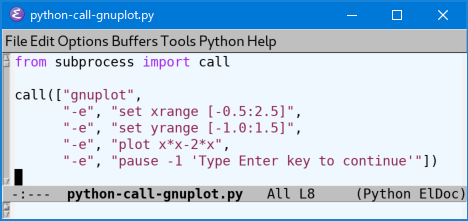
python-call-gnuplot.py
from subprocess import call

call(["gnuplot",
      "-e", "set xrange [-0.5:2.5]",
      "-e", "set yrange [-1.0:1.5]",
      "-e", "plot x*x-2*x",
      "-e", "pause -1 'Type Enter key to continue'"])
You can also use emacs to edit it.
Run python-call-gnuplot.py
python3 python-call-gnuplot.py
A Gnuplot X window is displayed.
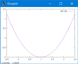
In X Terminal, type Enter key to continue.
Python Calls Gnuplot File Example
python-call-gnuplot-file.py
from subprocess import call

call(["gnuplot", "gnuplot.gnu"])
Run python-call-gnuplot-file.py
python3 python-call-gnuplot-file.py
gnuplot.gnu is executed and gnuplot.svg is generated as described in gnuplot.gnu
Python Matplotlib Plot Templates
We can use pyplot of matplotlib to plot figures in Python. If matplotlib was not yet installed, do the following:
pip3 install matplotlib
If install errors appear, download https://www.cygwin.com/setup-x86_64.exe and install matplotlib (View: Full; Search: matplotlib).
Python Matplotlib Plot Example
Below is a Python plot example. File name is pyplot.py. You can use emacs to edit it
import matplotlib.pyplot as plt
import numpy as np

x = np.linspace(-0.5, 2.5, 301) # 2.5-(-0.5)=3; 3k+1 points; k = 100 here
print (x) # x is a numpy array which has 301 elements

plt.plot(x, x*x-2*x, label="$x^2-2x$")
plt.legend(bbox_to_anchor=(0.5, 0.8), loc='center', borderaxespad=0, fontsize=10)
plt.savefig("pyplot.svg") # "pyplot.pdf"
Run pyplot.py
python3 pyplot.py
[-0.5  -0.49 -0.48 -0.47 -0.46 -0.45 -0.44 -0.43 -0.42 -0.41 -0.4  -0.39
 -0.38 -0.37 -0.36 -0.35 -0.34 -0.33 -0.32 -0.31 -0.3  -0.29 -0.28 -0.27
 -0.26 -0.25 -0.24 -0.23 -0.22 -0.21 -0.2  -0.19 -0.18 -0.17 -0.16 -0.15
 -0.14 -0.13 -0.12 -0.11 -0.1  -0.09 -0.08 -0.07 -0.06 -0.05 -0.04 -0.03
 -0.02 -0.01  0.    0.01  0.02  0.03  0.04  0.05  0.06  0.07  0.08  0.09
  0.1   0.11  0.12  0.13  0.14  0.15  0.16  0.17  0.18  0.19  0.2   0.21
  0.22  0.23  0.24  0.25  0.26  0.27  0.28  0.29  0.3   0.31  0.32  0.33
  0.34  0.35  0.36  0.37  0.38  0.39  0.4   0.41  0.42  0.43  0.44  0.45
  0.46  0.47  0.48  0.49  0.5   0.51  0.52  0.53  0.54  0.55  0.56  0.57
  0.58  0.59  0.6   0.61  0.62  0.63  0.64  0.65  0.66  0.67  0.68  0.69
  0.7   0.71  0.72  0.73  0.74  0.75  0.76  0.77  0.78  0.79  0.8   0.81
  0.82  0.83  0.84  0.85  0.86  0.87  0.88  0.89  0.9   0.91  0.92  0.93
  0.94  0.95  0.96  0.97  0.98  0.99  1.    1.01  1.02  1.03  1.04  1.05
  1.06  1.07  1.08  1.09  1.1   1.11  1.12  1.13  1.14  1.15  1.16  1.17
  1.18  1.19  1.2   1.21  1.22  1.23  1.24  1.25  1.26  1.27  1.28  1.29
  1.3   1.31  1.32  1.33  1.34  1.35  1.36  1.37  1.38  1.39  1.4   1.41
  1.42  1.43  1.44  1.45  1.46  1.47  1.48  1.49  1.5   1.51  1.52  1.53
  1.54  1.55  1.56  1.57  1.58  1.59  1.6   1.61  1.62  1.63  1.64  1.65
  1.66  1.67  1.68  1.69  1.7   1.71  1.72  1.73  1.74  1.75  1.76  1.77
  1.78  1.79  1.8   1.81  1.82  1.83  1.84  1.85  1.86  1.87  1.88  1.89
  1.9   1.91  1.92  1.93  1.94  1.95  1.96  1.97  1.98  1.99  2.    2.01
  2.02  2.03  2.04  2.05  2.06  2.07  2.08  2.09  2.1   2.11  2.12  2.13
  2.14  2.15  2.16  2.17  2.18  2.19  2.2   2.21  2.22  2.23  2.24  2.25
  2.26  2.27  2.28  2.29  2.3   2.31  2.32  2.33  2.34  2.35  2.36  2.37
  2.38  2.39  2.4   2.41  2.42  2.43  2.44  2.45  2.46  2.47  2.48  2.49
  2.5 ]
Generated pyplot.svg (nontransparent)

Python Matplotlib Plot X, Y Axes
pyplot_xy.py
import matplotlib.pyplot as plt
import numpy as np

x = np.linspace(-0.5, 2.5, 301) # 2.5-(-0.5)=3; 3k+1 points; k = 100 here
#print (x) # x is a numpy array which has 301 elements

# you can also use "fig, ax = plt.subplots()" to implement the followings
plt.gca().spines['top'].set_visible(False)        # do not show top spine
plt.gca().spines['right'].set_visible(False)      # do not show right spine
plt.gca().spines['bottom'].set_position(('zero')) # set position of x spine to y = 0
plt.gca().spines['left'].set_position(('zero'))   # set position of y spine to x = 0
plt.gca().set_xticks([-0.5,0.5,1.0,1.5,2.0,2.5])  # do not show 0.0 for x axis
plt.gca().set_yticks([-1.0,-0.5,0.5,1.0])         # do not show 0.0 for y axis
plt.gca().set_xticks(np.arange(-0.6,2.7,0.1), minor=True) # minor ticks
plt.gca().set_yticks(np.arange(-1.1,1.5,0.1), minor=True) # minor ticks

plt.plot(x, x*x-2*x, label="$x^2-2x$")
plt.legend(bbox_to_anchor=(0.5, 0.8), loc='center', borderaxespad=0, fontsize=10)
plt.savefig("pyplot_xy.svg") # "pyplot_xy.pdf"
Run pyplot_xy.py
python3 pyplot_xy.py
Generated pyplot_xy.svg (nontransparent)

Python Matplotlib Plot Time Complexity
BigOpyplot.py
import matplotlib.pyplot as plt
import numpy as np
import scipy.special as sp
import math

x = np.linspace(0.0000001, 10, 1001) # 0.0000001 != 0 for log2(); 10-0.0000001=10; 10k+1 = 1001

np.set_printoptions(precision=2, floatmode='fixed', suppress=True, threshold=np.inf) # print options
print(x) # x is a numpy array which has 1001 elements

plt.xticks(np.linspace(0, 10, 11))
plt.ylim(0.001, 10000)
plt.yscale('log')

y = np.log2(x)
plt.plot(x, y, "c", label="$\log_2(x)$")

#
#
# referring to the output figure, add your codes here
#
#

y = np.power(2, x)
plt.plot(x, y, "k", label="$2^x$")

y = sp.factorial(x)
plt.plot(x, y, label="$x!$")

# transparent plot and legend
plt.legend(bbox_to_anchor=(0.993, 0.01), loc='lower right', borderaxespad=0, fontsize=10, fancybox=True, framealpha=0.0)
plt.savefig("BigOpyplot.svg", transparent=True) # "BigOpyplot.pdf"
Run BigOpyplot.py
python3 BigOpyplot.py
[ 0.00  0.01  0.02  0.03  0.04  0.05  0.06  0.07  0.08  0.09  0.10  0.11
  0.12  0.13  0.14  0.15  0.16  0.17  0.18  0.19  0.20  0.21  0.22  0.23
  0.24  0.25  0.26  0.27  0.28  0.29  0.30  0.31  0.32  0.33  0.34  0.35
  0.36  0.37  0.38  0.39  0.40  0.41  0.42  0.43  0.44  0.45  0.46  0.47
  0.48  0.49  0.50  0.51  0.52  0.53  0.54  0.55  0.56  0.57  0.58  0.59
  0.60  0.61  0.62  0.63  0.64  0.65  0.66  0.67  0.68  0.69  0.70  0.71
  0.72  0.73  0.74  0.75  0.76  0.77  0.78  0.79  0.80  0.81  0.82  0.83
  0.84  0.85  0.86  0.87  0.88  0.89  0.90  0.91  0.92  0.93  0.94  0.95
  0.96  0.97  0.98  0.99  1.00  1.01  1.02  1.03  1.04  1.05  1.06  1.07
  1.08  1.09  1.10  1.11  1.12  1.13  1.14  1.15  1.16  1.17  1.18  1.19
  1.20  1.21  1.22  1.23  1.24  1.25  1.26  1.27  1.28  1.29  1.30  1.31
  1.32  1.33  1.34  1.35  1.36  1.37  1.38  1.39  1.40  1.41  1.42  1.43
  1.44  1.45  1.46  1.47  1.48  1.49  1.50  1.51  1.52  1.53  1.54  1.55
  1.56  1.57  1.58  1.59  1.60  1.61  1.62  1.63  1.64  1.65  1.66  1.67
  1.68  1.69  1.70  1.71  1.72  1.73  1.74  1.75  1.76  1.77  1.78  1.79
  1.80  1.81  1.82  1.83  1.84  1.85  1.86  1.87  1.88  1.89  1.90  1.91
  1.92  1.93  1.94  1.95  1.96  1.97  1.98  1.99  2.00  2.01  2.02  2.03
  2.04  2.05  2.06  2.07  2.08  2.09  2.10  2.11  2.12  2.13  2.14  2.15
  2.16  2.17  2.18  2.19  2.20  2.21  2.22  2.23  2.24  2.25  2.26  2.27
  2.28  2.29  2.30  2.31  2.32  2.33  2.34  2.35  2.36  2.37  2.38  2.39
  2.40  2.41  2.42  2.43  2.44  2.45  2.46  2.47  2.48  2.49  2.50  2.51
  2.52  2.53  2.54  2.55  2.56  2.57  2.58  2.59  2.60  2.61  2.62  2.63
  2.64  2.65  2.66  2.67  2.68  2.69  2.70  2.71  2.72  2.73  2.74  2.75
  2.76  2.77  2.78  2.79  2.80  2.81  2.82  2.83  2.84  2.85  2.86  2.87
  2.88  2.89  2.90  2.91  2.92  2.93  2.94  2.95  2.96  2.97  2.98  2.99
  3.00  3.01  3.02  3.03  3.04  3.05  3.06  3.07  3.08  3.09  3.10  3.11
  3.12  3.13  3.14  3.15  3.16  3.17  3.18  3.19  3.20  3.21  3.22  3.23
  3.24  3.25  3.26  3.27  3.28  3.29  3.30  3.31  3.32  3.33  3.34  3.35
  3.36  3.37  3.38  3.39  3.40  3.41  3.42  3.43  3.44  3.45  3.46  3.47
  3.48  3.49  3.50  3.51  3.52  3.53  3.54  3.55  3.56  3.57  3.58  3.59
  3.60  3.61  3.62  3.63  3.64  3.65  3.66  3.67  3.68  3.69  3.70  3.71
  3.72  3.73  3.74  3.75  3.76  3.77  3.78  3.79  3.80  3.81  3.82  3.83
  3.84  3.85  3.86  3.87  3.88  3.89  3.90  3.91  3.92  3.93  3.94  3.95
  3.96  3.97  3.98  3.99  4.00  4.01  4.02  4.03  4.04  4.05  4.06  4.07
  4.08  4.09  4.10  4.11  4.12  4.13  4.14  4.15  4.16  4.17  4.18  4.19
  4.20  4.21  4.22  4.23  4.24  4.25  4.26  4.27  4.28  4.29  4.30  4.31
  4.32  4.33  4.34  4.35  4.36  4.37  4.38  4.39  4.40  4.41  4.42  4.43
  4.44  4.45  4.46  4.47  4.48  4.49  4.50  4.51  4.52  4.53  4.54  4.55
  4.56  4.57  4.58  4.59  4.60  4.61  4.62  4.63  4.64  4.65  4.66  4.67
  4.68  4.69  4.70  4.71  4.72  4.73  4.74  4.75  4.76  4.77  4.78  4.79
  4.80  4.81  4.82  4.83  4.84  4.85  4.86  4.87  4.88  4.89  4.90  4.91
  4.92  4.93  4.94  4.95  4.96  4.97  4.98  4.99  5.00  5.01  5.02  5.03
  5.04  5.05  5.06  5.07  5.08  5.09  5.10  5.11  5.12  5.13  5.14  5.15
  5.16  5.17  5.18  5.19  5.20  5.21  5.22  5.23  5.24  5.25  5.26  5.27
  5.28  5.29  5.30  5.31  5.32  5.33  5.34  5.35  5.36  5.37  5.38  5.39
  5.40  5.41  5.42  5.43  5.44  5.45  5.46  5.47  5.48  5.49  5.50  5.51
  5.52  5.53  5.54  5.55  5.56  5.57  5.58  5.59  5.60  5.61  5.62  5.63
  5.64  5.65  5.66  5.67  5.68  5.69  5.70  5.71  5.72  5.73  5.74  5.75
  5.76  5.77  5.78  5.79  5.80  5.81  5.82  5.83  5.84  5.85  5.86  5.87
  5.88  5.89  5.90  5.91  5.92  5.93  5.94  5.95  5.96  5.97  5.98  5.99
  6.00  6.01  6.02  6.03  6.04  6.05  6.06  6.07  6.08  6.09  6.10  6.11
  6.12  6.13  6.14  6.15  6.16  6.17  6.18  6.19  6.20  6.21  6.22  6.23
  6.24  6.25  6.26  6.27  6.28  6.29  6.30  6.31  6.32  6.33  6.34  6.35
  6.36  6.37  6.38  6.39  6.40  6.41  6.42  6.43  6.44  6.45  6.46  6.47
  6.48  6.49  6.50  6.51  6.52  6.53  6.54  6.55  6.56  6.57  6.58  6.59
  6.60  6.61  6.62  6.63  6.64  6.65  6.66  6.67  6.68  6.69  6.70  6.71
  6.72  6.73  6.74  6.75  6.76  6.77  6.78  6.79  6.80  6.81  6.82  6.83
  6.84  6.85  6.86  6.87  6.88  6.89  6.90  6.91  6.92  6.93  6.94  6.95
  6.96  6.97  6.98  6.99  7.00  7.01  7.02  7.03  7.04  7.05  7.06  7.07
  7.08  7.09  7.10  7.11  7.12  7.13  7.14  7.15  7.16  7.17  7.18  7.19
  7.20  7.21  7.22  7.23  7.24  7.25  7.26  7.27  7.28  7.29  7.30  7.31
  7.32  7.33  7.34  7.35  7.36  7.37  7.38  7.39  7.40  7.41  7.42  7.43
  7.44  7.45  7.46  7.47  7.48  7.49  7.50  7.51  7.52  7.53  7.54  7.55
  7.56  7.57  7.58  7.59  7.60  7.61  7.62  7.63  7.64  7.65  7.66  7.67
  7.68  7.69  7.70  7.71  7.72  7.73  7.74  7.75  7.76  7.77  7.78  7.79
  7.80  7.81  7.82  7.83  7.84  7.85  7.86  7.87  7.88  7.89  7.90  7.91
  7.92  7.93  7.94  7.95  7.96  7.97  7.98  7.99  8.00  8.01  8.02  8.03
  8.04  8.05  8.06  8.07  8.08  8.09  8.10  8.11  8.12  8.13  8.14  8.15
  8.16  8.17  8.18  8.19  8.20  8.21  8.22  8.23  8.24  8.25  8.26  8.27
  8.28  8.29  8.30  8.31  8.32  8.33  8.34  8.35  8.36  8.37  8.38  8.39
  8.40  8.41  8.42  8.43  8.44  8.45  8.46  8.47  8.48  8.49  8.50  8.51
  8.52  8.53  8.54  8.55  8.56  8.57  8.58  8.59  8.60  8.61  8.62  8.63
  8.64  8.65  8.66  8.67  8.68  8.69  8.70  8.71  8.72  8.73  8.74  8.75
  8.76  8.77  8.78  8.79  8.80  8.81  8.82  8.83  8.84  8.85  8.86  8.87
  8.88  8.89  8.90  8.91  8.92  8.93  8.94  8.95  8.96  8.97  8.98  8.99
  9.00  9.01  9.02  9.03  9.04  9.05  9.06  9.07  9.08  9.09  9.10  9.11
  9.12  9.13  9.14  9.15  9.16  9.17  9.18  9.19  9.20  9.21  9.22  9.23
  9.24  9.25  9.26  9.27  9.28  9.29  9.30  9.31  9.32  9.33  9.34  9.35
  9.36  9.37  9.38  9.39  9.40  9.41  9.42  9.43  9.44  9.45  9.46  9.47
  9.48  9.49  9.50  9.51  9.52  9.53  9.54  9.55  9.56  9.57  9.58  9.59
  9.60  9.61  9.62  9.63  9.64  9.65  9.66  9.67  9.68  9.69  9.70  9.71
  9.72  9.73  9.74  9.75  9.76  9.77  9.78  9.79  9.80  9.81  9.82  9.83
  9.84  9.85  9.86  9.87  9.88  9.89  9.90  9.91  9.92  9.93  9.94  9.95
  9.96  9.97  9.98  9.99 10.00]
Generated BigOpyplot.svg (transparent)

Python Matplotlib Plot Data File
pyplot_data.py. It plots data from file latency.dat.
import matplotlib.pyplot as plt
import numpy as np

data = np.loadtxt('latency.dat')

plt.xlabel("Traffic load")
plt.ylabel("Latency (cycles)")

plt.plot(data[:,0], data[:,1], marker="o", markeredgewidth=0, label="Algo. 1 on workload 1")
plt.plot(data[:,0], data[:,2], marker="^", markeredgewidth=1, label="Algo. 2 on workload 1")
plt.plot(data[:,0], data[:,3], marker="D", markeredgewidth=0, label="Algo. 1 on workload 2")
plt.plot(data[:,0], data[:,4], marker="s", markeredgewidth=0, label="Algo. 2 on workload 2")

plt.legend(bbox_to_anchor=(0.3, 0.8), loc='center', borderaxespad=0, fontsize=10, fancybox=True, framealpha=0.0)
plt.savefig("pyplot_data.svg", transparent=True)
latency.dat
#1	2	3	4	5	col# gnuplot
#0	1	2	3	4	col# pyplot
#p	A11	A21	A12	A22
.05	285	270	312	288
.10	287	272	328	296
.15	291	275	338	308
.20	312	292	353	321
.25	347	323	370	339
.30	418	373	389	354
.35	487	418	402	369
.40	549	475	422	382
.45	613	523	436	401
.50	690	565	445	414
Run pyplot_data.py
python3 pyplot_data.py
Generated pyplot_data.svg (transparent)

Python Matplotlib Plot Bar Graph
pyplot_bar_graph.py
import matplotlib.pyplot as plt
import numpy as np

data = np.loadtxt('utilization.dat')

labels = ['BRU', 'IU', 'FPU', 'MUL', 'DIV', 'LSU']
plt.xticks([1,2,3,4,5,6],labels)
plt.ylim(0, 4)
plt.xlabel("CPU functional units (FUs)")
plt.ylabel("Number of functional units required")
width = 0.18

plt.bar(data[:,0]-0.3, data[:,1], width, label="1 thread")
plt.bar(data[:,0]-0.1, data[:,2], width, label="2 threads")
plt.bar(data[:,0]+0.1, data[:,3], width, label="4 threads")
plt.bar(data[:,0]+0.3, data[:,4], width, label="8 threads")

plt.legend(bbox_to_anchor=(0.2, 0.82), loc='center', borderaxespad=0, fontsize=10, fancybox=True, framealpha=0.0)
plt.savefig("pyplot_bar_graph.svg", transparent=True)
utilization.dat
#thread:1	2	4	8	# FUs
1	0.532	0.903	1.454	2.572	# BRU
2	0.444	0.753	1.213	2.145	# IU
3	0.750	1.258	2.035	3.538	# FPU
4	0.683	1.159	1.865	3.299	# MUL
5	0.264	0.448	0.721	1.276	# DIV
6	0.847	1.409	2.279	3.546	# LSU
Run pyplot_bar_graph.py
python3 pyplot_bar_graph.py
Generated pyplot_bar_graph.svg (transparent)

Python Matplotlib Plot Japanese
Japanese.py. It contains Japanese Hiragana, Katakana, Romaji, and Kanji.
# coding: utf-8

import matplotlib.font_manager as mfm
import matplotlib.pyplot as plt

#font_path = "/cygdrive/c/Windows/fonts/msmincho.ttc"
font_path = "/cygdrive/c/Windows/fonts/msgothic.ttc"
prop = mfm.FontProperties(fname = font_path)
plt.rcParams["pdf.fonttype"] = 42 # true type font

plt.text(0.30, 0.54, "おはよう、日本", fontproperties=prop, fontsize=20)
plt.text(0.33, 0.40, "NHK ニュース", fontproperties=prop, fontsize=20)

plt.savefig("Japanese.svg", transparent=True) # "Japanese.pdf"
Run Japanese.py
python3 Japanese.py
Generated Japanese.svg (transparent)

Plot Probability of Distributions on Python
Calculating the probabilities of the popular distribution functions can be done with the "scipy.stats" package easily. But here we just use the raw expressions of the distribution functions to calculate the probabilities.
You can change the parameter values of the distributions in the codes and draw your own curves.
If there is a run-time error like this,
RuntimeError: Failed to process string with tex because latex could not be foundyou may delete the line of "plt.text()" and the line(s) commented with "# latex".
正規分布 Normal Distribution
$\displaystyle P(x)={1\over{\sigma\sqrt{2\pi}}}e^{-{1\over{2}}\left({{x-\mu}\over\sigma}\right)^2}$
dist-normal.py
import matplotlib.pyplot as plt
import numpy as np
import math

plt.rc('text', usetex=True) # latex
plt.rc('text.latex', preamble=r'\usepackage{amsmath}') # latex

plt.title("Normal Distribution")
plt.xlabel("$x$")
plt.ylabel("Probability")
plt.xticks(np.linspace(-50, 50, 11))

x = np.arange(-50, 51) # x
mu = 0 # \mu

for sigma in range(5, 25, 5): # \sigma
    normal = (math.e)**(-((x-mu)/sigma)**2/2) / (sigma*(2*math.pi)**(0.5))
    plt.plot(x, normal, label="$\mu = {}, \sigma = {}$".format(mu,sigma))

plt.text(-50, 0.065, r'$\displaystyle P(x)={1\over{\sigma\sqrt{2\pi}}}e^{-{1\over{2}}\left({{x-\mu}\over\sigma}\right)^2}$', fontsize=15)

plt.legend(framealpha=0.0)
plt.savefig("dist-normal.svg", transparent=True)
#plt.show()
Run dist-normal.py
python3 dist-normal.py
Generated dist-normal.svg

離散一様分布 Discrete Uniform Distribution
$\displaystyle P(X=k)=\frac{1}{N}$
for $k=1,2,\cdots, N$.
dist-uniform.py
import matplotlib.pyplot as plt
import numpy as np

plt.rc('text', usetex=True) # latex

plt.title("Discrete Uniform Distribution")
plt.xlabel("$k$")
plt.ylabel("Probability")
plt.ylim(0, 0.3)

N = 6 # N
k = np.arange(1, N+1) # k
p = 1 / N # p

for i in k:
    plt.bar(i, p, label="$k={},\ N=6$".format(i))

plt.text(1.5, 0.25, r'$\displaystyle P(X=k)=\frac{1}{N}, \ k=1,2,\cdots, N$', fontsize=13)

plt.legend(framealpha=0.0)
plt.savefig("dist-uniform.svg", transparent=True)
# plt.show()
Run dist-uniform.py
python3 dist-uniform.py
Generated dist-uniform.svg

ベルヌーイ分布 Bernoulli Distribution
$\displaystyle P(X=k)= \left\{ \begin{array}{ll} 1-p&(k=0)\\ p&(k=1) \end{array} \right. $
for $k=0,1$.
dist-bernoulli.py
import matplotlib.pyplot as plt
import numpy as np

plt.rc('text', usetex=True) # latex

cases = [0.3, 0.5, 0.7] # p

plt.figure()
for i, p in enumerate(cases):
    plt.subplot(1, len(cases), i + 1)
    plt.subplots_adjust(wspace = 0.5)

    plt.bar(0, 1 - p, label="$1-p={:.1f}$".format(1-p)) # k = 0
    plt.bar(1, p, label="$p={:.1f}$".format(p))         # k = 1

    plt.xlabel("$k$")
    plt.ylabel("Probability")
    plt.xticks([0, 1])
    plt.ylim(0, 1)
    plt.legend(framealpha=0.0)

plt.suptitle("Bernoulli Distribution")
plt.savefig("dist-bernoulli.svg", transparent=True)
#plt.show()
Run dist-bernoulli.py
python3 dist-bernoulli.py
Generated dist-bernoulli.svg

幾何分布 Geometric Distribution
$\displaystyle P(X=k)=(1-p)^{k-1}p$
for $k = 1, 2, 3, \cdots$
dist-geometric.py
import matplotlib.pyplot as plt
import numpy as np

plt.rc('text', usetex=True) # latex

plt.title("Geometric Distribution")
plt.xlabel("$k$")
plt.ylabel("Probability")

k = np.arange(1, 11) # k

for p in np.linspace(0.2, 0.8, 3): # p
    geometric = (1 - p)**(k - 1) * p
    plt.plot(k, geometric, "-o", label="$p = {}$".format(p))

plt.text(3, 0.7, r'$\displaystyle P(X=k)=(1-p)^{k-1}p$', fontsize=13)

plt.legend(framealpha=0.0)
plt.savefig("dist-geometric.svg", transparent=True)
#plt.show()
Run dist-geometric.py
python3 dist-geometric.py
Generated dist-geometric.svg

二項分布 Binomial Distribution
$\displaystyle P(X=k)=\binom{n}{k}p^k(1-p)^{n-k}$
for $k = 0, 1, 2, \cdots, n$
If $n = 1$, it becomes Bernoulli Distribution (ベルヌーイ分布).
dist-binomial.py
import matplotlib.pyplot as plt
import numpy as np
import math

plt.rc('text', usetex=True) # latex
plt.rc('text.latex', preamble=r'\usepackage{amsmath}') # latex

plt.title("Binomial Distribution")
plt.xlabel("$n$")
plt.ylabel("Probability")

p = 0.5 # p
n = np.arange(0, 71) # n
binomial = np.zeros(71, dtype=float)

for k in range(5, 25, 5): # k
    for j in n:
        if j >= k:
            binomial[j] = p**k * (1-p)**(j-k) * math.factorial(j) / (math.factorial(k)*math.factorial(j-k))
        else:
            binomial[j] = 0.0
    plt.plot(n, binomial, "-o", label="$p = {}$, $k = {}$".format(p,k))

plt.text(14, 0.21, r'$\displaystyle P(X=k)=\binom{n}{k}p^k(1-p)^{n-k}$', fontsize=13)

plt.legend(framealpha=0.0)
plt.savefig("dist-binomial.svg", transparent=True)
#plt.show()
Run dist-binomial.py
python3 dist-binomial.py
Generated dist-binomial.svg

ポアソン分布 Poisson Distribution
$\displaystyle P(X=k)=\frac{\lambda^ke^{-\lambda}}{k!}$
for $k = 0, 1, 2, \cdots$
Here we show how to use the "scipy.stats" package to draw the probability of the Poisson distribution. You may install scipy:
pip3 install scipy
dist-poisson.py
import matplotlib.pyplot as plt
import scipy.stats as stats # scipy.stats
import numpy as np

plt.rc('text', usetex=True) # latex

plt.title("Poisson Distribution")
plt.xlabel("$k$")
plt.ylabel("Probability")

k = np.arange(0, 36) # k

for lmd in range(5, 25, 5): # \lambda
    poisson = stats.poisson.pmf(k,lmd) # poisson probability mass function
    plt.plot(k, poisson, "-o", label="$\lambda = {}$".format(lmd))

plt.text(8, 0.145, r'$\displaystyle P(X=k)=\frac{\lambda^ke^{-\lambda}}{k!}$', fontsize=20)

plt.legend(framealpha=0.0)
plt.savefig("dist-poisson.svg", transparent=True)
#plt.show()
Run dist-poisson.py
python3 dist-poisson.py
Generated dist-poisson.svg

パスカルの三角形 Pascal Triangle
pascal_triangle.py
print("input the number n (n < 20): ", end="")
n = int(input())
if n > 19:
    n = 19

for i in range (0, n+1):
    print("n = {:2d}".format(i), end="")
    for j in range (0, n-i):
        print("   ", end="")
    coef = 1
    for j in range (0, i+1):
        print("{:6d}".format(coef), end="")
        coef = coef * (i - j) // (j + 1)
    print("")
Run pascal_triangle.py
python3 pascal_triangle.py
input the number n (n < 20): 11
n =  0                                      1
n =  1                                   1     1
n =  2                                1     2     1
n =  3                             1     3     3     1
n =  4                          1     4     6     4     1
n =  5                       1     5    10    10     5     1
n =  6                    1     6    15    20    15     6     1
n =  7                 1     7    21    35    35    21     7     1
n =  8              1     8    28    56    70    56    28     8     1
n =  9           1     9    36    84   126   126    84    36     9     1
n = 10        1    10    45   120   210   252   210   120    45    10     1
n = 11     1    11    55   165   330   462   462   330   165    55    11     1
LaTeX Documentation Templates
LaTeX is widely used in preparing documentations and publications such as books, journal/conference papers, technical reports, theses/dissertations, etc. Below is a figure that will be embedded into the LaTeX document.
LaTeX Gnuplot Figure
m1dxm1m1.gnu
unset border
set nokey

set encoding utf8
set minussign

set xrange [-6:6.2]
set yrange [-6:6.6]

set xtics axis
set ytics axis

set xtics -6, 1, 6
set ytics -6, 1, 6

set xtics font "Times-Roman, 14"
set ytics font "Times-Roman, 14"

set xtics add ('' 0)
set ytics add ('' 0) offset -1, 0.1

set arrow 1 from -6.3,0 to 6.5,0 linetype -1
set arrow 2 from 0,-6.3 to 0,6.9 linetype -1

plot -1/(x-1)-1 with line

set terminal pdf
set output "m1dxm1m1.pdf"
replot
Run m1dxm1m1.gnu
gnuplot m1dxm1m1.gnu
Generated m1dxm1m1.pdf
LaTeX Report Example
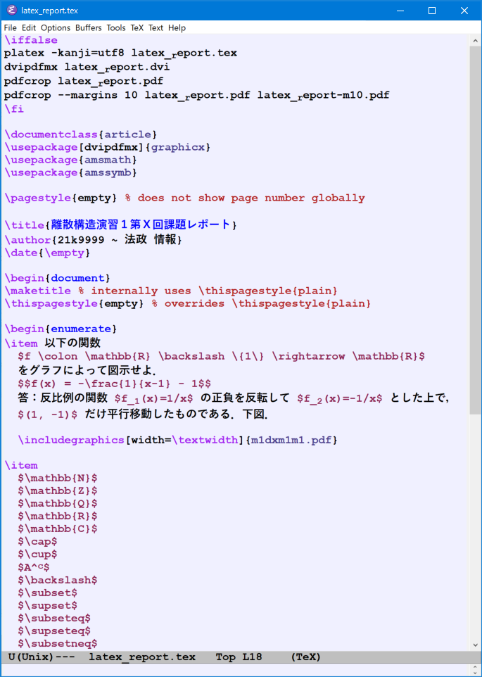
latex_report.tex
\iffalse
platex -kanji=utf8 latex_report.tex
dvipdfmx latex_report.dvi
pdfcrop latex_report.pdf
pdfcrop --margins 10 latex_report.pdf latex_report-m10.pdf
\fi

\documentclass{article}
\usepackage[dvipdfmx]{graphicx}
\usepackage{amsmath}
\usepackage{amssymb}

\pagestyle{empty} % does not show page number globally

\title{離散構造演習1第X回課題レポート}
\author{21k9999 ~ 法政 情報}
\date{\empty}

\begin{document}
\maketitle % internally uses \thispagestyle{plain}
\thispagestyle{empty} % overrides \thispagestyle{plain}

\begin{enumerate}
\item 以下の関数
  $f \colon \mathbb{R} \backslash \{1\} \rightarrow \mathbb{R}$
  をグラフによって図示せよ.
  $$f(x) = -\frac{1}{x-1} - 1$$
  答:反比例の関数 $f_1(x)=1/x$ の正負を反転して $f_2(x)=-1/x$ とした上で,
  $(1, -1)$ だけ平行移動したものである.下図.

  \includegraphics[width=\textwidth]{m1dxm1m1.pdf}

\item
  $\mathbb{N}$
  $\mathbb{Z}$
  $\mathbb{Q}$
  $\mathbb{R}$
  $\mathbb{C}$
  $\cap$
  $\cup$
  $A^c$
  $\backslash$
  $\subset$
  $\supset$
  $\subseteq$
  $\supseteq$
  $\subsetneq$
  $\supsetneq$
  $\not\subset$
  $\not\supset$
  $\nsubseteq$
  $\nsupseteq$
  $\in$
  $\notin$
  $\pi$
  $\sqrt{-7}$
  $<$
  $>$
  $\leq$
  $\geq$
  $\nless$
  $\ngtr$
  $\nleq$
  $\ngeq$
  $\frac{123}{11}$
  $\displaystyle\frac{123}{11}$
  $\sum_{i=0}^{n-1}2^i$
  $\displaystyle\sum_{i=0}^{n-1}2^i$
  $\binom{n}{k}$
  $\displaystyle\binom{n}{k}$
  $\emptyset$
  $\varnothing$
  $\circ$ $\bigcirc$
  $\not\mathrel{R}$
  $\equiv$
  $\neq$
  $\gg$
  $\ll$
  $\succ$
  $\prec$
  $\times$
  $\infty$
  $\bigtriangleup$
  $$v_y=gt$$
  $$s=\int_0^tv_y\ dt=\int_0^tgt\ dt=\frac{1}{2}gt^2$$
\end{enumerate}

\end{document}
You can edit the latex file also with emacs, as shown below. There is a character 'U' in the left bottom corner. It indicates the encoding of the current file. 'U' stands for UTF8; 'S' stands for Shift-JIS; and 'E' stands for EUC.
Generate PDF
platex -kanji=utf8 latex_report.tex
dvipdfmx latex_report.dvi
Generated latex_report.pdf
Remove the white margins of PDF pages
pdfcrop latex_report.pdf
Generated latex_report-crop.pdf
Keep extra margins
pdfcrop --margins 10 latex_report.pdf latex_report-m10.pdf
Note: the unit is bp. 72 bp = 1 inch. 29 bp is approximately 1 cm.
Generated latex_report-m10.pdf
Try to comment out the \maketitle and re-generate the PDF.
More about LaTeX ...
Read more for LaTeX.